Capital and labour markets - IMACLIM
| Corresponding documentation | |
|---|---|
| Previous versions | |
| Model information | |
| Model link | |
| Institution | Centre international de recherche sur l'environnement et le développement (CIRED), France, http://www.centre-cired.fr., Societe de Mathematiques Appliquees et de Sciences Humaines (SMASH), France, http://www.smash.fr. |
| Solution concept | General equilibrium (closed economy) |
| Solution method | SimulationImaclim-R is implemented in Scilab, and uses the fonction fsolve from a shared C++ library to solve the static equilibrium system of non-linear equations. |
| Anticipation | Recursive dynamics: each year the equilibrium is solved (system of non-linear equations), in between two years parameters to the equilibrium evolve according to specified functions. |
Capital markets
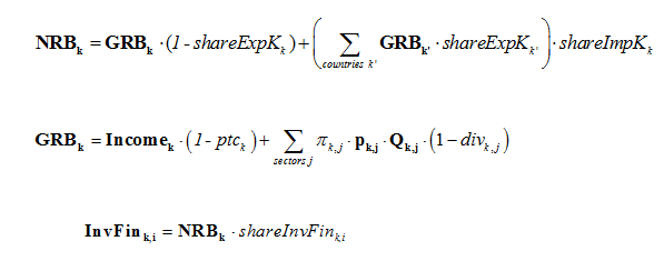
A share (shareExpK) of gross domestic savings (GRB) is internationally tradable, and distributed via an international capital pool. Each regions receives a share of the international pool (shareImpK). In the default model setting, both shares (shareExpK and shareImpK) are exogenous: shareExpK is exponentially reduced such that international financial imbalances disappear by 2050 and shareImpK remains constant throughout the simulation period.
The remaining share of domestic savings and imported capital (NRB) are then invested in each region respectively.
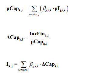
The total amount of money InvFink,i available for investment in sector i in the region k allows new capacities DCapk,i to be constructed at a cost pCapk,i (equation 9-3-5). The cost pCapk,i depends on the quantities βj,i,k and the prices pIk,j of goods j required by the construction of a new unit of capacity in sector i and in region k. Coefficient βj,i,k is the amount of good j necessary to constuct the equipment corresponding to one new unit of production capacity in sector i of the region k. Finally, in each region, the total demand for goods for building new capacities is given by the last equation below.
Each sector anticipates future production levels through an anticipation of future prices and demand and formulates the corresponding investment demand. Total available investment Ik,j is then distributed among sectors according to their demand.
Labour markets
At each time step, producers operate in static equilibria with a fixed input of labor per unit of output. This labor input, corresponding to labor productivity, evolves between two yearly equilibria following exogenous trends in labor productivity.
Three of the model features explain the possibility of under-utilization of labor as a factor of production, and thus unemployment. First, rigidity of real wages, represented by a wage curve can prevent wages falling to their market-clearing level. Put another way, instantaneous adjustment of wages to the economic context in the static equilibrium does not occur in an optimal manner. Second, in the static equilibrium, the fixed technologies (Leontief coefficients even for labor input) prevent substitution among production factors in the short run. And third, the installed productive capital is not mobile across sectors, which creates rigidities in the reallocations of production between sectors when relative prices change.
In each region k, each sector employs the labor force lk,i.Qk,i, where lk,i is the unitary labor input (in hours worked) and Qk,i the production. The underutilization of the labor force, equivalently referred to as the 'unemployment rate' in the following, _zk is therefore equal to one minus the ratio of the employed labor force across all sectors over Lk, the total labor force:
Obviously, this definition of the unemployment rate is a limitation of the current calibration of the model. Future developments will look into the possibility to differentiate labor markets per regions. However, one important difficulty lies in the lack of reliable data on the underutilization of the labor forces in all regions, in particular due to informal economy, very diverse accounting rules for unemployment rates and variations in hours worked per person across countries. No endogenous mobility of workers between regions is accounted for in the model. Thus twelve separate labor markets are represented.
We chose to model labor market imperfections through an aggregate regional wage curve that links real wage levels to the unemployment rate. This representation is based on labor theories developed in the 1980s and early 1990s in which an aggregate wage curve, or wage setting curve, is the primary distinguishing feature (an overview can be found in Layard et al., 2005layard2005unemployment; Lindbeck, 1993lindbeck1993unemployment; or Phelps, 1992phelps1992consumer). The novel approach of these models, when introduced, was to replace the conventional labor supply curve with a negatively-sloped curve linking the level of wages to the level of unemployment. The interpretation of this wage curve is given either by the bargaining approach (Layard and Nickell, 1986)layard1986unemployment or the wage-efficiency approach (Shapiro and Stiglitz, 1984)shapiro1984equilibrium. Both interpretations rely on the fact that unemployment represents an outside threat that leads workers to accept lower wages the greater the threat. The bargaining approach emphasizes the role of workers' (or union) power in the wage setting negotiations, power that is weakened when unemployment is high. The wage-efficiency approach takes the firms' point of view and assumes that firms set wage levels so as to discourage shirking; this level is lower when the threat of not finding a job after being caught shirking gets higher. The wage curve specification allows the theories to be consistent with both involuntary unemployment and the fact that real wages fluctuate less than the theory of the conventional flexible labor supply curve predicts. Microeconometric evidence for such formulations was given in a seminal contribution by (Blanchflower and Oswald 1995)blanchflower1994introduction.
In practice, the wage curve for each region k in our model is implemented through the relation:
where w is the hourly nominal wage level, pind the consumption price index, z the unemployment rate, ref indexes represent the values of the variables at the calibration date, pindref is derived from the final consumption prices and volumes at the calibration date, wref is calibrated from the total salaries per sector in the GTAP 6 database (Reference?) and the shares of labor force per sector are taken from International Labor Organisation statistics. By default, aw is calibrated to 1 and evolves in parallel to labor productivity so that unitary real wages are indexed on labor productivity. zref represents the underutilization of the labor force at the calibration date. f is a function equal to one when the unemployment rate is equal to its calibration level, and is negatively sloped, representing a negative elasticity of wages level to unemployment [3]. Choosing a functional form and calibrating the function is particularly tricky, notably due to the lack of reliable data to fully inform the functioning of the labor markets worldwide. We chose a function of the form a.(1-tanh(c.z)), and calibrate the parameters a and c so as to have the desired value and elasticity at the calibration point.
By default, we assume all regions' labor markets to be identical and set the underutilization of the labor force at 10% (Contrary to the definition by the U.S. Bureau of Labor Statistics, the level of unemployment is expressed here in terms of worked hours and not in terms of persons)[4] and the wage curve elasticity at -0.1 for all regions (This is a value emerging from many econometric studies, e.g. (Blanchflower and Oswald 1995)blanchflower1994introduction, (Blanchflower and Oswald 2005). Guivarch et al. (2011)guivarch2011costs analyzes the critical role of labour markets imperfections, and in particular of the value of the wage curve elasticity, on the formation of climate stabilization costs.


