Economic activity - TIAM-UCL
| Corresponding documentation | |
|---|---|
| Previous versions | |
| Model information | |
| Model link | |
| Institution | University College London (UCL), UK, https://www.ucl.ac.uk. |
| Solution concept | Partial equilibrium (price elastic demand) |
| Solution method | Linear optimisation |
| Anticipation | Perfect Foresight
(Stochastic and myopic runs are also possible) |
GDP
Estimations of future economic growth are much more uncertain than future population growth. Few studies exist that forecast GDP up to 2100 and so unlike population assumptions, GDP figures in TIAM-UCL are not based on a single source. Economic growth rates have been compared to assumptions made for scenarios in the 4th assessment report of the IPCC (Tsuneyuki 1999) and Clarke et al. (2007). Global GDP is assumed to grow from $50 trillion in 2010 to $155 trillion in 2050 and $350 trillion in 2100 (all GDP are in 2005 US$). Current figures for 2010 have been taken from the IMF (2009).
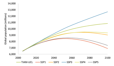
Figures for future economic growth are based on an approximate assumption of economic convergence between regions (see Figure 3 5), i.e. that low income regions grow faster compared to high income regions. The figure shows this convergence of per capita income among world regions. The GDP per person is calculated as the ratio of GDP and population. The economic convergence is a central point in the assumptions on socio-economic drivers. The effect becomes clear when one compares the GDP per head in different regions. In 2005 India is the poorest region with a GDP per head of 10% of the world average and the USA is the richest region with 600% of the world average. In 2100 this picture changes with India having a GDP per head that has now grown to 55% of the world average and the USA being the richest country with 350% of the world average.
GDP growth rates are expected to decline over the course of the 21st century, while they remain higher for developing countries than for developed countries. Owing to the shrinking population, the growth rates for South Korea and Japan are very low and turn negative at the end of the 21st century. Growth rates for Western Europe, the UK and the United States are assumed to drop from an average of 2.2% to 1.3% p.a. in 2050. The only region that is expected to increase GDP growth rates over the first decades is Africa based on a growing population and its current low income levels. Global economic growth is approximately in the mid-range of the growth in the SSP scenarios
<figure id="fig:GDP per capita">
 </figure>
Sectoral drivers
The industrial, services and agricultural sectors have different growth drivers from all other sectors i.e. they are not directly related to growth in GDP and a decoupling factor. There are a number of reasons for this, but key is that there is expected to be a decoupling of growth in, for example, production of steel and growth in GDP that is cannot be trivially estimated by a single decoupling factor. Additionally, the industrial service demands can be interpreted as represent the production of physical quantities e.g. tonnes of steel, tonnes of aluminium etc. Projections of future production are provided by various sources, who look in detail at the array of factors that affect production and consumption levels on regional basis. These sources therefore likely provide more robust estimates of future production while also providing a more tangible projection of what is being estimated.
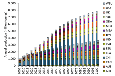
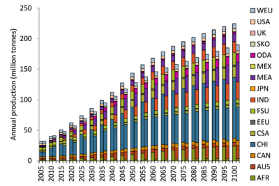
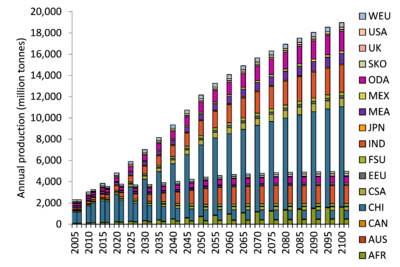
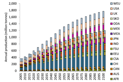
The projections of steel, aluminium and cement, paper and chemicals production globally used in TIAM-UCL are provided in the Figures below. These figures also shows how these compare with the projections used in ETSAP-TIAM. These quantities have been estimated using the regional per-capita consumption and productions projections from IEA up to 2050 ensuring that these balance on a global level). A single provider was used for this estimation to ensure consistency across the different metallic and non-metallic sectors. Consumption from 2050 to 2100 was then based on historical trends in per-capita consumption from 2000 to 2050, so, for example, annual aluminium consumption is assumed to trend towards 35 kg/person and steel towards 500 kg/capita as regions increase their GDP/capita. Energy-service demands rely on production and not consumption levels, which are not equal because of trade. Production to satisfy this increasing demand was thus estimated by projecting trends in production between 2010 and 2050 whilst again ensuring that consumption and production matched on a global level.
It can be seen that the new projections are in general lower than those used previously, particularly in the case of cement. These projections can be easily modified to account for different socio-economic scenarios, for example if it is assumed that material intensity will be greater or lower in the future (included within the main assumptions of the SSPs for example). The energy-service demand for agriculture is derived in a similar manner. A relationship is given between crop caloric demand/capita, protein demand/capita, and GDP/capita. This suggests that both follow an approximate square root relationship with GDP/capita (so if GDP/capita doubles protein demand and crop calorie demand increase by 41%).
TIAM-UCL requires the energy-service demand and the energy intensity of protein and crop calories are very different. However, because both crop and protein demand follow a similar relationship to GDP/capita, the GDP/capita assumption shown in the crop Figure can be used to estimate how total consumption within each region will change in the future demand. This therefore assumes a constant ratio of crop to meat calories in all regions in the future, although clearly because GDP/capita increases, the absolute level of each also increases over time. Again production levels are required for energy-service demands and not consumption. A strong assumption is therefore made whch is that the current (2005) ratio of production to consumption would remain constant in the future, a ratio that varies significantly between different regions. This assumption and projections of consumption and production can be easily modified to account for different socio-economic scenarios, say if it is assumed that global trade of agricultural goods will increase or decrease in the future.
<figure id="fig:steel">
 </figure>
<figure id="fig:aluminium">
 </figure>
<figure id="fig:cement">
 </figure>
<figure id="fig:paper">
 </figure>
