Land-use - IMACLIM
| Corresponding documentation | |
|---|---|
| Previous versions | |
| Model information | |
| Model link | |
| Institution | Centre international de recherche sur l'environnement et le développement (CIRED), France, http://www.centre-cired.fr., Societe de Mathematiques Appliquees et de Sciences Humaines (SMASH), France, http://www.smash.fr. |
| Solution concept | General equilibrium (closed economy) |
| Solution method | SimulationImaclim-R is implemented in Scilab, and uses the fonction fsolve from a shared C++ library to solve the static equilibrium system of non-linear equations. |
| Anticipation | Recursive dynamics: each year the equilibrium is solved (system of non-linear equations), in between two years parameters to the equilibrium evolve according to specified functions. |
This section presents the land-use module of IMACLIM-R. This model is currently run independently of IMACLIM-R. The linkage to IMACLIM-R is in progress. The version 1.0 of the land-use model is extensively described in Souty et al. (2012)souty2012nexus(open access).
Modelling strategy
The Nexus Land-Use model (NLU) is designed to represent the processes of global agricultural intensification, which are viewed as being a key factor in the resolution of the conflicts on land-use. NLU provides a bioeconomic modelling framework that ensures consistency between economic behaviors and spatial biophysical constraints at the global level. Global land area is divided into 12 regions (see section Spatial process), and 6 land-use types: forests, 2 croplands types and 3 pasture types.
The representation of the production system is chosen to account for various biophysical features as well as agronomic practices. This representation relies on three main components: (i) a detailed representation of the livestock production system, based on the Bouwman et al. (2005)bouwman2005exploring model; (ii) potential crop yields, from the Lund-Postdam-Jena dynamic global vegetation model for managed Land (LPJmL, Bondeau et al.,2007)bondeau2007modelling; and, (iii) a non-linear biomass production function, mimicking the crop yield response function to inputs (such as nitrogen fertilizers).
Such a modelling strategy implies that among the four main factors of production of the agricultural sector: (i) land, (ii) chemical inputs and their associated embodied energy, (iii) labor and (iv) capital; that the former two are modelled in detail while the latter two are not. As a consequence, NLU is better suited to dealing with land-use and energy-related issues, including the effects of carbon pricing than it is for, for example, for sketching the consequences of agricultural intensification on labor markets. Land-fertilizer substitution is a core mechanism of the model, as this process is seen to be a major driver of future agricultural changes. This is because of the trends in rising fertilizer prices spurred by tensions on the fossil energy and phosphorus markets. Irrigation is incorporated into the model by differentiation of the potential yields of rainfed and irrigated lands.
The economic principles governing farmer decisions used in the NLU follow from Ricardian rent theory (Ricardo, 1817)ricardo1817foreign. In line with this theory, we consider that the poorer lands are the last to be cultivated. In the NLU modelling framework, the Ricardian frontier represents a dividing line between an intensive agricultural system, composed of a mosaic of crops and pastures, and an extensive agricultural system, exclusively composed of pastures. In the model the line moves as the former progressively expands into the latter as the demand for land rises. Hence, unlike the original Ricardian vision in which the agricultural system reacts to a growing demand for land by expanding the size of arable lands into natural ecosystems, adjustments occur from reallocations inside the boundaries of the already exploited land between intensive and extensive agriculture. This vision is consistent with the report made by Bouwman et al. (2005)bouwman2005exploring that "most of the increase in meat and milk production during the past three decades has been achieved by increasing production in mixed and industrial production systems and much less so in pastoral systems. Despite the fast increase of ruminant production by 40% in the 1970--1995 period, the global area of grassland has increased by only 4 %".
Model functioning
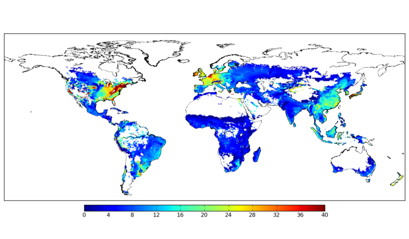
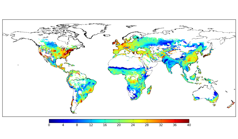
For the base year (2001), a representative potential yield is computed at the scale of a 0.5°×0.5° grid from the potential yields given for 11 crop functional types (CFT) by the vegetation model LPJmL. Grid points with the same potential yield are grouped together in land classes. The actual yield of each land class is a function of the chemical inputs used, such as fertilizers and pesticides. This yield-fertilizer function is characterized by decreasing returns, with the potential yield as asymptote. In each land class, the consumption of chemical inputs and the associated yield are determined by cost minimization. The yield/fertilizer relationship is calibrated using fertilizer consumption values (Nitrogen, Phosphorus, Potassium) calculated from FAOSTAT data (FAO, 2013)grubler2010technological. It can also be calibrated on GTAP 6 values as done in Souty et al. (2012)souty2012nexus. Two of the parameters of the yield-fertilizer relationship -minimum yield and slope at the origin- are calibrated so as to minimize the error between modeled and observed crop yields over the 1961- 2006 period. Nitrogen application via manure and leguminous crop residues are implicitly considered in the calibration of the yield-fertiliser function.
Following Bouwman et al. (2005)fao1, the livestock production system is divided into an extensive and an intensive production system. The extensive production system produces only grass-fed ruminants. The intensive production system includes both ruminants and monogastrics (non-grazing animals). In the intensive production system, ruminants are fed with a mix of grass, food crops, residues, fodder and other roughages. In both systems, grass is assumed to come from permanent pastures that can be grazed or cut for hay where permanent pastures are defined according to the Food and Agriculture Organization nomenclature. Two types of permanent pastures, intensive and extensive, are distinguished according to the system to which they provide grass. Monogastric animals are fed with food crops, residues and fodder and animal products. Fodder for monogastric and intensive ruminants is grown on cropland. Croplands are assumed to be located exclusively on the most productive lands including pastures feeding the intensive production system. Conversely, the extensive pastures are located on the least productive lands. This split of agricultural land we carry out does not completely fit with the data since a sizeable share of today?s extensive pastures belong to land classes with high-yields. Therefore, we consider an additional category of extensive pastures, which we call residual pastures.
Each type of land-use; forest, cropland, intensive, extensive and residual pastures, is distributed among the land classes, giving for each land class of potential yield the area fractions of forest, cropland, intensive, extensive and residual pastures. At each time step, NLU calculates a global supply/demand balance from exogenous data on total calorific consumption of food crops for agrofuels, plant foods (food crops for humans), ruminants and monogastric products. The total land supply for agriculture, excluding croplands not represented in LPJmL, is deduced from the exogenously set annual evolution i.e. increase or decrease, of the forest area.
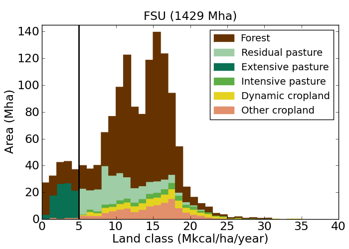
In NLU the agricultural sector, with one representative farmer per land class, minimizes hs production costs under two constraints, (i) land availability and (ii) a global resource-use balance of plant food and ruminant calories. To do this minimization, the representative farmer can substitute both cropland for fertilizer input and extensive livestock production for intensive. There is a link between both these two types of substitution, as the intensification in crop production (i.e. substituting cropland for fertilizer) (i) makes the production of feed for animals more profitable, but on the other hand (ii) mitigates the pressure on land and thus reduces the scarcity rent. The former effect benefits the intensive system and the latter benefits the extensive one. The combination of these two effects determines the exact repartition and position of the Ricardian frontier between the intensive and extensive production systems.
<figure id="fig:imaclim_7">
</figure>
When the level of profit of the intensive system increases relative to the extensive one, the Ricardian production frontier moves to land classes with lower fertility (the black vertical bar moves to the left in <xr id="fig:imaclim_7"/>) and the corresponding extensive pastures becomes part of the intensive system. In the opposite case, the frontier moves to more fertile land classes and the extensive system increases at the expense of the intensive one. The cropland-fertilizer substitution elasticity is not parameterized, but is derived from a cost-minimization program. Its value decreases as the Ricardian production frontier moves towards less productive lands, where it becomes less profitable to substitute land for fertiliser.
The shadow price of land (= land rent) is endogenously computed in the NLU model, as the lagrangian multiplier associated with the land constraint in the cost-minimization program. Fertilizer prices are driven by an econometric equation in which the explanatory variables are the exogenous variations of oil, gas and industry prices provided by the energy modules of IMACLIM-R (currently not linked to the NLU module).
The hypothesis of a single representative agent means neglecting the differences between different farms and different situations and assuming they are all characterized by the same potential yield in a given region. The difference between farm types, especially farms of different sizes, however, is not very problematic, as (Chavas, 2008)chavas2008economics has shown that long run economies of scale in terms of land-use are small.
NLU balances edible biomass resources and their use, in physical terms. Data is obtained from the FAO and is expressed in kilocalories (kcal), which is the common unit used to represent nutrition (1 kcal=4.1868 kJ). For the model base year (2001), the resource-use balance is established using data from the global agriculture database, Agribiom (Dorin, 2011)dorin2011agribiom. Using calories makes it possible to deal with different types of biomass for human consumption. In NLU, plant food, ruminant and monogastric calories are thus separated, and each type of calories is associated with a specific production process.
International trade is modelled by using a pooled representation of product flows without any consideration of the geographic origin of products. The value of imports and exports are determined by relative regional calorie prices, taking into account a simple representation of imperfect competition and food sovereignty considerations. Regions can trade food crops with each other as well as ruminant products (the trade of monogastric products is held constant).
Due to data availability constraints, two categories of crops are distinguished in NLU: (i) "dynamic" crops, modeled in LPJmL which correspond to most cereals, oilseeds, sugar beet and cassava, and a small share of fodder crops and (ii) "other" crops, not modeled in LPJmL, which correspond to sugar cane, palm oil, fruits and vegetables , some fodder crops and remaining crops. "Dynamic" crop yield is determined endogenously, by taking into account the amount of fertiliser used and biophysical constraints . The share of "other" crops in total crop production is assumed to be constant over the projection period 2005-2050. The "other" crop yield is an exogenous parameter calculated based on projections from Alexandratos and Bruinsma (2012)alexandratos2012world.
In 2001 (model base year), the land area use is based on the land-use map from Ramankutty et al. (2008)ramankutty2008farming. The total cropland area amounts to 1472 Mha, divided between 748 Mha of "dynamic" crops and 724 Mha of "other" crops. Production on "dynamic" cropland represents 75% of the global calorie production reported by the global database Agribiom.
Model equations
All the model equations are discribed in Souty et al. (2012)souty2012nexus (open access).
Main input data
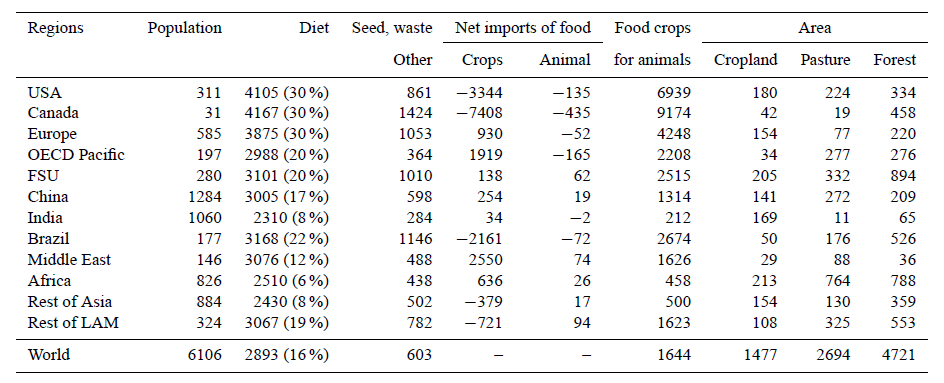
Table 1: Main input data for each region of the model for the base year, 2001. Cropland and pasture areas (in Mha) are taken from Ramankutty et al. (2008)ramankutty2008farming and forests areas (in Mha) are from Poulter et al. (2011)poulter2011plant, while other data are from Agribiom (Dorin, 2011)dorin2011agribiom. Population is in millions. Diet is calorie consumption in kcal per capita and per day with the fraction of animal products in consumption in brackets. Consumption of seed, agricultural waste at the farm level and other food crops used in the production of lubricants and cosmetics in kcal/capita/day. Net imports of food crops and animal products in kcal/capita/day. Food crops used as feed in kcal kcal/capita/day (Sect. 5.4). 1 kcal=4.1868 kJ.
<figure id="fig:imaclim_8">
</figure>
<figure id="fig:imaclim_9">
</figure>
Other input data (land distribution of potential yields, crop aggregates, feed conversion factors of monogastrics and ruminants, consumed grass yield...) can be found in Souty et al. (2012)souty2012nexus.
Evaluation of the model performances
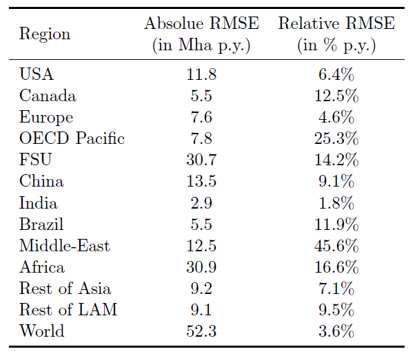
The performance of the model is investigated by undertaking a backcasting exercise for the period 1961-2006. Estimations of cropland areas in each region are evaluated against historical data in each region from Ramankutty and Foley (1999)ramankutty1999estimating. Results are shown in Table 2. At the global scale, the simulated cropland area matches the measured cropland rather well. The root-mean-square errors (RMSE) amounts to 52.3 Mha p.a. in absolute terms and 3.6% p.a. in relative ones. The model performs well for half of the modelled regions (USA, Europe, China, India, Rest of Asia, Rest of Latin America), with a RMSE in absolute terms lower than 10% p.a.. The difference between estimations and measured data is more substantial for Canada, Former Soviet Union (FSU), Brazil and Africa, with RMSEs ranging from 11.9% p.a. to 16.6% p.a. However, the NLU fails to accurately model the evolution of cropland area for OECD Pacific (RMSE = 25.3% p.a.) and for the Middle-East (RMSE = 45.6% p.a.). For some regions the model does not explain or reproduce some structural changes visible from the measured data. For instance, for the FSU, the increase in fertilizer input before the collapse of the USSR was not matched by a corresponding yield increases. In OECD Pacific, yields decreased with fertilizer increase for many years, a phenomena the model cannot reproduce either.
Table 2: Root-mean square errors (RMSE) of simulated cropland area against observations over the period 1961-2006.
There is no systematic over- or under- estimation bias for the model, as cropland areas are rather under-estimated in half of the regions (Canada, Europe, India, Rest of LAM, Brazil, China), while they are rather over-estimated in the other half (USA, OECD, Pacific, MiddleEast, Africa, Rest of Asia).
Overall, the modelled evolution of cropland areas appears to be more variable than the measured cropland data. A possible explanation for this could be public intervention and price stabilization. For a number of decades, the use of industrial fertilizers has been largely subsidized, directly or indirectly, in many regions of the world. These subventions, as well as interventions in commodity markets, contributed to the stabilization of farmers revenues. In fertilizer price statistics, subsidies are deducted wherever possible, thus, the fertilizer price provided by the World Bank does probably not correspond to the actual price paid by farmers. This would thus introduce errors in our simulations over historic periods. Fertilizer subsidies have however been progressively suppressed since the 80's/90's. Therefore, we can expect such errors to have less influence in future simulations.
