Production system and representation of economic sectors - GRACE
Firms are assumed to supply goods and services to maximise their subject to production technologies in perfect competitive markets. Production technologies are described by nested separable constant elasticity of substitution (CES) functions (see below), and inputs are divided into primary input factors (i.e., labour, capital and resources) and intermediate inputs from each sector. Output and the use of all input factors are subject to taxation, reported in the database. Production of primary energy includes natural resources as a sector-specific production factor, with a fixed supply.
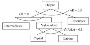
Two forms of the nested CES functions are adopted by the core version of the GRACE model. Figure 2.3 illustrates the structure of the functional forms for production of primary energy – crude oil, coal, and gas. The parameters starting with small letter “e” indicate the elasticities of substitution (the same for figures illustrating structures of nested functions below). At the top-level, output is described by a standard CES function of the value-added-intermediates aggregate and the natural resource. The substitution elasticity at the top-level as well as the value share of natural resource determine the price elasticity of supply of fossil fuels. In the basic version of the GRACE model, this substitution elasticity is set to 0.3. At the second level, the value-added-intermediates aggregate is depicted by a Leontief function (with no substitution) of intermediates and the value-added aggregate. The value-added aggregate is a standard CES function of capital and labour. The substitution elasticity between capital and labour is another important parameter, which determines technological flexibilities in production. The empirical literature typically rejects the hypothesis of a Cobb-Douglas function, where the substitution elasticity between capital and labour equals 1, and shows that the elasticity tends to be less than unity (Arrow et al., 1961). In the core version of the GRACE model, we assume a substitution elasticity of 0.3.
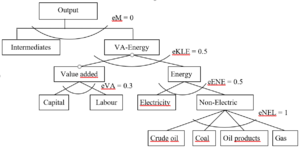
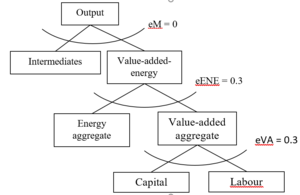
The other form of production functions illustrated in Figure 2.4 is for production of goods/services other than primary energy – crude oil, coal, and gas. Output is described assuming no substitution (Leontief function) between intermediates and the value-added-energy aggregate. At the second level, the value-added-energy aggregate is a standard CES function of the energy aggregate and the value-added aggregate, with a substitution elasticity of 0.5. The energy aggregate is formed from a CES function of electricity and non-electric energy inputs. The aggregate of non-electric energy inputs is depicted by a Cobb-Douglas function (elasticity of substitution = 1) of coal, crude oil, oil products, and natural gas. The elasticities of substitution at all nests are adopted from the MIT EPPA model (Paltsev et al., 2005).
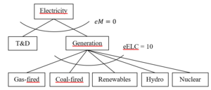
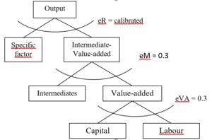
In later studies that focus on the energy sector, we employ a more elaborated structure for the power generation sector. The calibration of the power generation sector is based on the GTAP9-Power database, which is an electricity-detailed extension of Version 9 of the GTAP database (Aguiar et al., 2016; Peters, 2016). The GTAP9-Power database depicts the global economy in 2011 and provides data on 140 regions and 68 commodities. In the GRACE model, the power generation sector is divided into the five sub-sectors gas-fired plants, coal-fired plants, nuclear power, hydropower and renewables (see Figure 2.5 and 2.6a, b).
The power generation sector consists of generation, and transmission and distribution (T&D). Transmission and distribution are represented by a service sector, which is consumed in a fixed proportion relative to power generation, as described by a Leontief function (Peters, 2016b). Following many other CGE-based studies (e.g., Peters, 2016b; Sue Wing, 2008; Wing, 2006), we assume imperfect substitutability among technologies to depict market inertias associated with switching from one technology to another. Hence, a stricter climate policy will lead to substitution towards less carbon intensive technologies, without ending up with corner solutions. The choice of elasticity is subject to a compromise between a high elasticity to reflect the homogeneity of the output, and a low elasticity to reflect the incompleteness in switches between technologies.
Following Paltsev et al. (2005), we incorporate a technology-specific factor on the supply side of power generation from renewables, nuclear power, and hydro power. This can be interpreted as a natural resource constraint. The specific factor is assumed substitutable with the value added, meaning that we calibrate the substitution elasticity to achieve an assumed price elasticity of supply. There are only a few empirical estimates of the price elasticity of the supply of renewable electricity generation. For example, Johnson (2011) estimated a value of 2.7 for the price elasticity pertaining to the supply of renewables in the USA. This value was used by Paltsev et al. (2005) and Rivers (2013). In our analysis, we use the same value for renewables, whereas for nuclear power and hydropower, we use a value of 1 for the price elasticity of supply.
| Corresponding documentation | |
|---|---|
| Previous versions | |
| No previous version available | |
| Model information | |
| Model link | |
| Institution | Center for International Climate Research (CICERO), Norway, https://cicero.oslo.no/en. |
| Solution concept | General equilibrium (closed economy) |
| Solution method | SimulationRecursive dynamic solution method |
| Anticipation | |
