Transport - IMACLIM
| Corresponding documentation | |
|---|---|
| Previous versions | |
| Model information | |
| Model link | |
| Institution | Centre international de recherche sur l'environnement et le développement (CIRED), France, http://www.centre-cired.fr., Societe de Mathematiques Appliquees et de Sciences Humaines (SMASH), France, http://www.smash.fr. |
| Solution concept | General equilibrium (closed economy) |
| Solution method | SimulationImaclim-R is implemented in Scilab, and uses the fonction fsolve from a shared C++ library to solve the static equilibrium system of non-linear equations. |
| Anticipation | Recursive dynamics: each year the equilibrium is solved (system of non-linear equations), in between two years parameters to the equilibrium evolve according to specified functions. |
Modeling the dynamics of the transportation sector
In static equilibrium, the transport of passengers and merchandise are characterized by the following parameters:
- The number and charachteristics of households personal vehicles,
- The efficiency of the fleet of personal vehicles,
- The physical capacities of the different modes of transport,
- The coefficients of intermediary energy use in the transport sectors,
- The coefficients of intermediary consumption of transport in all sectors.
In the recursive dynamic structure of Imaclim-R the "transport" dynamic module represents the evolutions of these parameters.
Waisman et al. (2013)waisman2012th give a detailed description of the representation of the transportation sector in Imaclim-R, and analyze the sector's role in the development of low-carbon pathways. The section below gives a description of the representation of the dynamics of the sector in Imaclim-R.
Personal vehicles: stock and energy intensity
The evolution in the rate of motorization in each region has been found to be strongly linked to the evolution of average income per inhabitant and to the distribution of income in the population. It is however only slightly sensitive to variations in fuel prices (Storchmann, 2005)storchmann2005long. The representation of these links in IMACLIM-R are based upon the SMP model, a sectorial model of energy use in the transport sector developed in a collaboration between the International Energy Agency and the World Energy Council (Fulton and Eads, 2004)fulton2004iea. The key feature of the SMP model is that it uses an income elasticity that varies depending on the rate of motorization. In practice this means an elasticity that varies with income. Regional variation resulting from historical and geographical factors, mean that the correlation between an absolute level of wealth and the possession of a vehicle is not transposable from one region to another. The saturation effect on the possession of personal vehicles thus appears at a level of average income that depends on the region.
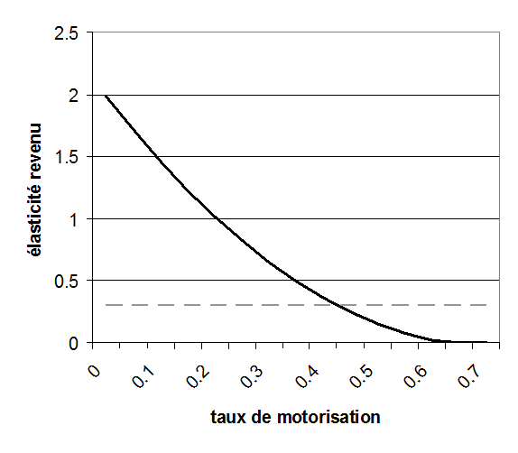
The income elasticity, αk, is linked to the rate of motorization according to a formula adapted from the SMP model and schematized in <xr id="fig:imaclim_3"/>. In the regions where the annual average income (measured in purchasing power parity) does not exceed $5000 per capita, this elasticity is maintained equal to 0.3 regardless of the rate of motorization, in order to represent the threshold effects linked to accessing auto-mobility in today's least developed economies. By multiplying Cars_pc by the total population one obtains the total size of the car fleet, denoted CARS. The size of the personal vehicle fleet, CARS, then determines the capacity of transport associated with the automobile mode, a parameter which is taken into account in the budget-time constraint of households in static equilibrium.
<figure id="fig:imaclim_3">
</figure>
The efficiency of the automobile fleet depends both upon technical progress and upon technological choices households make upon acquisition of their vehicles. In the model the automobile fleet is charachterised by different generations of vehicles categorised according to the year in which they were put into service and further grouped into four types of vehicles: conventional or hybrid with, in both cases, standard or improved technology. This schematic representation, includes contrasting characteristics for the four types of vehicles : purchase price, energy efficiency and fixed and variable maintenance costs. All costs are calibrated with data from the International Energy Agency (IEA, 2006)iea2 and evolve over time in resopnce to technical progress. Hybrid vehicle technology is assumed to improve so as to make possible consumption levels in the order of 1.5 litres per 100 kilometres. This figure can also be understood as being an average of electrical vehicles and rechargeable hybrid vehicles.
At every time step, 'the technological composition of the new generation of vehicles' results from the households' choosing from among the four specific technologies. This choice is carried out by comparing, for each of the four available vehicle technologies, the levelised average cost associated with the production of a vehicle-kilometre. This average cost is calculated using technological characteristics of the different types of vehicles in a manner similar to that used in calculating the complete cost of the technologies used to produce electricity. In doing so it is assumed that households formulate a myopic view of the trajectory of future energy prices, that is to say, they consider that future prices will be equal to those of the preceding static equilibrium. In the case where an explicit carbon policy in introduced, it is assumed that households anticipate perfectly future values of the tax and add it to their myopic scenario of energy prices. The levelized average production cost of a vehicle-kilometer for a specific technology, denoted TECH in the following, is obtained using Equation 1 by summing up the fixed and variable costs linked to the possession and usage of the vehicle respectively. The fixed costs are made up of the levelized purchase cost (denoted CINV_carsk,TECH) and the annual fixed running costs associated with the possession of a vehicle (e.g. insurance).Both fixed and running costs are normalised to a kilometre covered on the basis of a hypothesis on the annual average distance covered by vehicles (denoted average_km_per_yeark) applied to each region on. Variable costs group the fuel costs which depend both on the anticipated final price scenarios (denoted _p_fuel_anticip_taxed_cars_) and the fuel consumption of the vehicle type per vehicle.kilometre (denoted sym). In all of these calculations, the discount rate adopted by the households, denoted disck,CAR, is fixed as a scenario hypothesis between 0.12 and 0.18, according to the region.
with:
The market shares of each new vehicle technology is obtained by a logit function which makes it possible to take into account heterogeneities in household choices and the coexistence on the market of several different vehicle types (Clarke and Edmonds, 1993)clarke1993modelling:
These shares are then allocated to the new generation of vehicles, denoted CAR_new, obtained by the difference between the new total size of the CARS fleet and the old depreciated fleet.
Finally, the new average energy intensity of automobile transport (expressed in Mtoe per passenger.kilometre) is obtained by taking into account the composition of the fleet and the levels of use of the different generations and types of vehicles:
This equation includes two behavioural parameters drawn from the SMP model which are necessary togo from the theoretical energy use levels for the four types of vehicles to the average energy intensity of the whole fleet per passenger.kilometer: (1) the average occupation rate of the vehicles, denoted occupancyk, and (2) the relationship between the theoretical energy use level of the vehicles and actual observed energy use level, denoted on_road_gap_factork.
Other means of transport: capacities and energy use
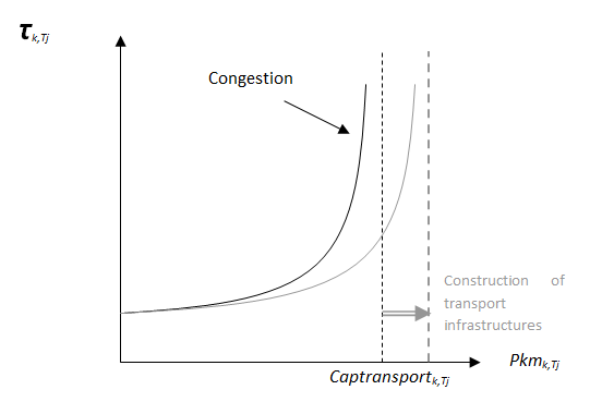
The evolution of passenger transport capacity is directly linked to the evolution in transport infrastructures that follows from public and private sector decisions. By default, these public and private sector decisions finance capacity evolution in responce to demand increases either explicitly through state spending on road infrastructures or via the investment decisions of the respective transport sectors. The evolution in the levels of capacity then modifies the 'time-efficiency' of the different transport modes used in the calculation of the time-budget constraint in the households' utility maximization program in the static equilibrium (<xr id="fig:imaclim_4"/>).
<figure id="fig:imaclim_4">
</figure>
The non-automobile transport intermediary energy use respond to reduced, simple forms of efficiency improvement:
- In the air sector, fuel use declines by 0.7% per year due to autonomus technical progress that includes both advances in airplane design and the improved use of flight and destination organizational measures aimed at filling plane seats.
- In the maritime sector, intermediary energy use per unit of transport remains unchanged.
- In the which includes sector of freight and passenger transport by land, the average use of liquid fuels evolves in response to a price elasticity of fuels, denoted elast_Et_OTk, which is fixed at -0.3 but does not go below an asymptote fixed at 25% of its initial level (See Equation 5). This aggregated representation is a preliminary step towards a more detailed representation of this sector divided into sub-sectors. In fact, in the present version of the model, the sector 'public land transport' groups road and rail freight and road (bus) and rail passenger transport. This level of aggregation follows directly from the GTAP data format upon which the model is calibrated. This format does not distuinguish different sub-sectors of transport. The dynamic evolution of the energy use of this sector is thus a function of vehicle technological progress, modal shifts (particularly shifts in freight between road and rail) and modifications in the structural composition of the sector arising from changes in the relative weights of the comprising sub-sectors.
Evolution in the transport demand of other sectors
Production technologies used in each sector are described using Leontief functions. The functions have fixed levels of labor, energy and other intermediary inputs. This means that at a given point in time, that the transport demand of production sectors in each of the three freight transportation modes (air, water and land ) is measured by input-output coefficients, FjIC, which describe a linear dependence in a given mode of freight transport, j, to production volumes.
The input-output coefficients, FjIC, capture implicitly (a) the spatial organization of the production processes in terms of specialization/concentration of production units and (b) the constraints imposed on distribution in terms of distance to markets and just-in-time processes, and these two factors drive the modal breakdown and the intensity of demand for freight mobility. The input-output coefficients can evolve exogenously over time to capture assumptions on changes in the energy efficiency of freight vehicles, in the logistic organization of the production/distribution process and in the modal breakdown.
For enterprises making organizational and production decisions an uncertainty exists regarding their reaction to variations in the price of transport however small. Therefore it has been decided to fix the evolution of these parameters exogenously. In the default model setting, these coefficients of intermediate consumption of transport by sectors are maintained constant. This is in line with observed historical tendencies.


