Modelling of climate indicators - IMACLIM: Difference between revisions
m (Text replacement - "(Image:.*IMPORT\/attachments\/[0-9]*\/[0-9]*.png\|)" to "File:") |
Eoin OBroin (talk | contribs) No edit summary |
||
| (4 intermediate revisions by the same user not shown) | |||
| Line 14: | Line 14: | ||
=== Carbon Cycle Model and Climate Model === | === Carbon Cycle Model and Climate Model === | ||
The carbon cycle is a three-box model, after Nordhaus and Boyer (2010). The model is a linear three-reservoir model (atmosphere, biosphere + ocean mixed layer, and deep ocean). Each reservoir is assumed to be homogenous (well-mixed in the short run) and is characterized by a residence time inside the box and corresponding mixing rates with the two other reservoirs (for longer timescales). Carbon flows between reservoirs depend on constant transfer coefficients. GHGs emissions (CO<sub>2</sub> solely) accumulate in the atmosphere and are slowly removed by biospheric and oceanic sinks. | The carbon cycle is a three-box model, after Nordhaus and Boyer (2010)[[CiteRef::nordhaus2003warming]]. The model is a linear three-reservoir model (atmosphere, biosphere + ocean mixed layer, and deep ocean). Each reservoir is assumed to be homogenous (well-mixed in the short run) and is characterized by a residence time inside the box and corresponding mixing rates with the two other reservoirs (for longer timescales). Carbon flows between reservoirs depend on constant transfer coefficients. GHGs emissions (''CO<sub>2</sub>'' solely) accumulate in the atmosphere and are slowly removed by biospheric and oceanic sinks. | ||
The stocks of carbon (in the form of CO<sub>2</sub>) in the atmosphere, in the biomass and upper ocean, and in the deep ocean are, respectively, A, B, and O. The variable E is the CO<sub>2</sub> emissions. The evolution of A, B, and O is given by | The stocks of carbon (in the form of ''CO<sub>2</sub>'') in the atmosphere, in the biomass and upper ocean, and in the deep ocean are, respectively, ''A'', ''B'', and ''O''. The variable ''E'' is the ''CO<sub>2</sub>'' emissions. The evolution of ''A'', ''B'', and ''O'' is given by | ||
[[File:35815687.png]] | [[File:35815687.png]] | ||
| Line 22: | Line 22: | ||
The fluxes are equal to<br />[[File:35815688.png]] | The fluxes are equal to<br />[[File:35815688.png]] | ||
The initial values of A, B, and O, and the parameters a12, a21, a23, and a32 determine the fluxes between reservoirs. The main criticism which may be addressed to this Carbon-cycle model is that the transfer coefficients are constant. In particular, they do not depend on the carbon content of the reservoir (e.g. deforestation hindering biospheric sinks) nor are they influenced by ongoing climatic change (e.g. positive feedbacks between climate change and the carbon cycle). | The initial values of ''A'', ''B'', and ''O'', and the parameters ''a12'', ''a21'', ''a23'', and ''a32'' determine the fluxes between reservoirs. The main criticism which may be addressed to this Carbon-cycle model is that the transfer coefficients are constant. In particular, they do not depend on the carbon content of the reservoir (e.g. deforestation hindering biospheric sinks) nor are they influenced by ongoing climatic change (e.g. positive feedbacks between climate change and the carbon cycle). | ||
Nordhaus | Nordhaus' original calibration has been adapted to reproduce both; data until 2010 and; results from the IMAGE model for a given trajectory of ''CO<sub>2</sub>'' emissions. This gives the following results (for a yearly time step): ''a12''= 0.02793, ''a21''=0.03427, ''a23''=0.007863, ''a32''=0.0003552, with the initial conditions: ''A''2010=830 ''GtC'' (i.e. 391ppm), ''B''2010=845 ''GtC'' and ''O''2010=19254 ''GtC''. The additional forcing caused by ''CO<sub>2</sub>'' and ''non-CO<sub>2</sub>'' gases is given by | ||
[[File:35815689.png]] | [[File:35815689.png]] | ||
where A<sub>PI</sub> is the pre-industrial CO<sub>2</sub> concentration (280 ppm), F<sub>2x</sub> is the additional radiative forcing for a doubling of the CO<sub>2</sub> concentration (3.71 W.m^-2^), and F<sub>non-CO2</sub> is the additional radiative forcing of non-CO<sub>2</sub> gases. | where ''A<sub>PI</sub>'' is the pre-industrial ''CO<sub>2</sub>'' concentration (280 ppm), ''F<sub>2x</sub>'' is the additional radiative forcing for a doubling of the ''CO<sub>2</sub>'' concentration (3.71 W.m^-2^), and ''F<sub>non-CO2</sub>'' is the additional radiative forcing of ''non-CO<sub>2</sub>'' gases. | ||
The temperature model is a two-box model, after Schneider and Thompson (1981) and Ambrosi | The temperature model is a two-box model, after Schneider and Thompson (1981)[[CiteRef::schneider1981atmospheric]] and Ambrosi et al. (2003)[[CiteRef::ambrosi2009optimal]], with the atmosphere temperature ''T<sub>A</sub>'' and the ocean temperature ''T<sub>O</sub>'' as follows: | ||
[[File:35815690.png]] | [[File:35815690.png]] | ||
where T2x is the equilibrium temperature increase at the doubling of the CO<sub>2</sub> concentration, that is, it represents climate sensitivity. All parameters have been calibrated to reproduce results from CMIP5 from CNRM-CERFACS global climate model, CNRM-CM5, over the 21st century for RCP3-PD and RCP4.5 radiative forcing trajectories (using a least squares method). This calibration leads to the following parameter values for heat transfer rates (for a yearly time step): | where ''T2x'' is the equilibrium temperature increase at the doubling of the ''CO<sub>2</sub>'' concentration, that is, it represents climate sensitivity. All parameters have been calibrated to reproduce results from CMIP5 from CNRM-CERFACS global climate model, CNRM-CM5, over the 21st century for RCP3-PD and RCP4.5 radiative forcing trajectories (using a least squares method). This calibration leads to the following parameter values for heat transfer rates (for a yearly time step): ''σ1''= 0.054''C.W<sup>-1</sup>-1.m<sup>2</sup>'', ''σ2''= 0.664 ''C.W<sup>-1</sup>-1.m<sup>2</sup>'' and ''σ3''= 0.0308, and a climate sensitivity of 2.6°C. | ||
Latest revision as of 18:09, 14 December 2016
| Corresponding documentation | |
|---|---|
| Previous versions | |
| Model information | |
| Model link | |
| Institution | Centre international de recherche sur l'environnement et le développement (CIRED), France, http://www.centre-cired.fr., Societe de Mathematiques Appliquees et de Sciences Humaines (SMASH), France, http://www.smash.fr. |
| Solution concept | General equilibrium (closed economy) |
| Solution method | SimulationImaclim-R is implemented in Scilab, and uses the fonction fsolve from a shared C++ library to solve the static equilibrium system of non-linear equations. |
| Anticipation | Recursive dynamics: each year the equilibrium is solved (system of non-linear equations), in between two years parameters to the equilibrium evolve according to specified functions. |
Modelling of Climate indicators
The impact of emissions scenarios on climate indicators is computed using a simplified 3-box carbon cycle model and a simplified 2-box climate model (Ambrosi, 2003).
Radiative Forcing from Other Gases
The radiative forcing from other gases are taken as exogenous assumptions.
Carbon Cycle Model and Climate Model
The carbon cycle is a three-box model, after Nordhaus and Boyer (2010)nordhaus2003warming. The model is a linear three-reservoir model (atmosphere, biosphere + ocean mixed layer, and deep ocean). Each reservoir is assumed to be homogenous (well-mixed in the short run) and is characterized by a residence time inside the box and corresponding mixing rates with the two other reservoirs (for longer timescales). Carbon flows between reservoirs depend on constant transfer coefficients. GHGs emissions (CO2 solely) accumulate in the atmosphere and are slowly removed by biospheric and oceanic sinks.
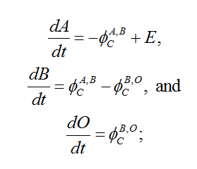
The stocks of carbon (in the form of CO2) in the atmosphere, in the biomass and upper ocean, and in the deep ocean are, respectively, A, B, and O. The variable E is the CO2 emissions. The evolution of A, B, and O is given by
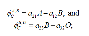
The initial values of A, B, and O, and the parameters a12, a21, a23, and a32 determine the fluxes between reservoirs. The main criticism which may be addressed to this Carbon-cycle model is that the transfer coefficients are constant. In particular, they do not depend on the carbon content of the reservoir (e.g. deforestation hindering biospheric sinks) nor are they influenced by ongoing climatic change (e.g. positive feedbacks between climate change and the carbon cycle).
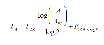
Nordhaus' original calibration has been adapted to reproduce both; data until 2010 and; results from the IMAGE model for a given trajectory of CO2 emissions. This gives the following results (for a yearly time step): a12= 0.02793, a21=0.03427, a23=0.007863, a32=0.0003552, with the initial conditions: A2010=830 GtC (i.e. 391ppm), B2010=845 GtC and O2010=19254 GtC. The additional forcing caused by CO2 and non-CO2 gases is given by
where API is the pre-industrial CO2 concentration (280 ppm), F2x is the additional radiative forcing for a doubling of the CO2 concentration (3.71 W.m^-2^), and Fnon-CO2 is the additional radiative forcing of non-CO2 gases.
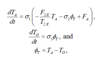
The temperature model is a two-box model, after Schneider and Thompson (1981)schneider1981atmospheric and Ambrosi et al. (2003)ambrosi2009optimal, with the atmosphere temperature TA and the ocean temperature TO as follows:
where T2x is the equilibrium temperature increase at the doubling of the CO2 concentration, that is, it represents climate sensitivity. All parameters have been calibrated to reproduce results from CMIP5 from CNRM-CERFACS global climate model, CNRM-CM5, over the 21st century for RCP3-PD and RCP4.5 radiative forcing trajectories (using a least squares method). This calibration leads to the following parameter values for heat transfer rates (for a yearly time step): σ1= 0.054C.W-1-1.m2, σ2= 0.664 C.W-1-1.m2 and σ3= 0.0308, and a climate sensitivity of 2.6°C.


